当前位置:网站首页>D1 understanding neural networks from zero
D1 understanding neural networks from zero
2022-07-20 17:39:00 【Poppy679】
# Loda Data & Data Analysis
from sklearn.datasets import load_boston

dataset = load_boston()# load the dataset
dir(dataset)# show the form of the dataset
dataset['feature_names']# show the tag of the dataset

# we can see the introdcution about these tags by print(dataset['CRIM'])
# define the problem
# if you are the state salesman,you have to konw the price of the state
# (given some description data about the state to konw its price)

import pandas as pd
# pandas means panel data set Panel data -excel Data processing - Easier programming

dataframe = pd.DataFrame(dataset['data']) # put the dataset into the pd
# we can use dataframe.head() to show up how many data we have
# use len(dataframe) to see the total number of the dataset
# only input the dataframe can output 10

dataframe.columns = dataset['feature_names']# show the name of all the columns
dataframe['price'] = dataset['target'] # can show the price of these states
# and the name "price" is rename from "target"
dataframe

# What's the most significant(salient) feature of the house price?
%matplotlib inline
dataframe.corr()# caculate the relation of these data

# use print(dataset['DESCR']) can show the descrblie of these tags
import seaborn as sns # the tool about Data visualization
sns.heatmap(dataframe.corr(),annot = True, fmt = '.1f') #  The darker the color, the less relevant

#  Based on the above analysis , It is found that the number of bedrooms in the house is most positively correlated with the price of wine
#  simple : How to estimate the area of a house according to the number of bedrooms ?

# 1970S An idea :save the data
X_rm = dataframe['RM'].values
Y = dataframe['price'].values

# Do dictionary mapping
rm_to_price = {
    r:y for r, y in zip(X_rm,Y)}
rm_to_price
rm_to_price[5.727]#  When the input data cannot be found in the dictionary , You're going to report a mistake

import numpy as np
#  therefore , When the input data cannot be found in the dictionary , You can find the closest data in the dictionary and output its value
def find_price_by_similar(history_price,query_x, topn=3):
    #  Sort the houses , according to x and sorted Sort by distance , Take the closest value when outputting
    # return np.mean([p for x, p in sorted(history_price.items(),key = lambda x_y:(x_y[0] - query_x)**2)[:topn]])
    most_similar_items = sorted(history_price.items(),key=lambda e:(e[0] - query_x)**2)[:topn]
    most_similar_prices = [price for rm, price in most_similar_items]
    average_prices = np.mean(most_similar_prices)

    return average_prices

find_price_by_similar(rm_to_price,7)
such , When the input value is not in the data set tag in , It will take something close to its value tag As output .
K-Neighbor-Nearest =>KNN
Very classic machine learning algorithm . KNN The method is inefficient , When processing a large amount of data ( There are other questions )
# A More Efficient Learning Method
# if we can find the relationship between X_rm and y
# every time when we want to caculate ,input the function ,and we get the predicted value
import matplotlib.pyplot as plt
plt.scatter(X_rm,Y)#  Draw a scatter diagram , Visual display x,y The relationship between

x And y The relationship becomes y=kx+b, In fact, it is the best k and b, Find the best fitting effect
What is called good fitting effect ?
How to evaluate the relationship between the predicted value and the actual value , Which prediction is better ?
You need to define a function :Loss function ( Mean square error :MSE)
L o s s ( y , y ^ ) = 1 n ∑ i ∈ N ( y i ^ − y i ) 2 Loss(y, \hat{y}) = \frac{1}{n} \sum_{i \in N} (\hat{y_i} - y_i) ^ 2 Loss(y,y^)=n1i∈N∑(yi^−yi)2
for instance : call loss function , The closer the value is. 0, It shows that the effect is better
real_y = [3,6,7]
y_hats = [3,4,7]
y_hats_2 = [3,6,6]

def loss(y,y_hat):
    return np.mean((np.array(y) - np.array(y_hat))**2)
loss(real_y,y_hats)
loss(real_y,y_hats_2)#  comparison yhats_2 better
Find the best k and b
Method 1, Calculate directly by calculus .( Least square method )
Method 2, Use the method of random simulation to calculate
import random
VAR_MAX,VAR_MIN = 100,-100

min_loss = float('inf')
best_k,best_b = None,None

def model(x,k,b):
    return x * k + b

total_times = 100 #  The number of iterations 100

for t in range(total_times):
    k,b = random.randint(VAR_MIN,VAR_MAX),random.randint(VAR_MIN,VAR_MAX)
    loss_ = loss(Y,model(X_rm,k,b))
    print("i'm looking for~")#  You can see , Constantly looking for good k/b value
    #  At first , The update will be more popular 、 frequent ; As the number of iterations increases , The update is getting slower and slower
    if loss_ < min_loss:
        min_loss = loss_
        best_k,best_b = k,b
        print(' stay {} At this moment, I found a better k:{} and b:{}, Now loss yes :{}'.format(t,k,b,loss_))
In this way, we can observe what is found in each iteration k and b value .
Show by image , You can observe the linear model obtained by fitting
plt.scatter(x, y)
plt.scatter(x, [best_k * rm + best_b for rm in x])

How to make updates faster ?
Monte Carlo simulation
Usually, Monte Carlo simulation solves various mathematical problems by constructing random numbers that conform to certain rules . For those problems that are too complex to obtain analytical solutions or have no analytical solutions at all , Monte Carlo simulation is an effective method to obtain numerical solutions . Generally, the most common application of Monte Carlo simulation in mathematics is Monte Carlo integration .
Supervisor
L o s s ( k , b ) = 1 n ∑ i ∈ N ( ( k ∗ r m i + b ) − y i ) 2 Loss(k, b) = \frac{1}{n} \sum_{i \in N} ((k * rm_i + b) - y_i) ^ 2 Loss(k,b)=n1i∈N∑((k∗rmi+b)−yi)2
∂ l o s s ( k , b ) ∂ k = 2 n ∑ i ∈ N ( k ∗ r m i + b − y i ) ∗ r m i \frac{\partial{loss(k, b)}}{\partial{k}} = \frac{2}{n}\sum_{i \in N}(k * rm_i + b - y_i) * rm_i ∂k∂loss(k,b)=n2i∈N∑(k∗rmi+b−yi)∗rmi
∂ l o s s ( k , b ) ∂ b = 2 n ∑ i ∈ N ( k ∗ r m i + b − y i ) \frac{\partial{loss(k, b)}}{\partial{b}} = \frac{2}{n}\sum_{i \in N}(k * rm_i + b - y_i) ∂b∂loss(k,b)=n2i∈N∑(k∗rmi+b−yi)
Code implementation :
def partial_k(k, b, x, y):
    return 2 * np.mean((k * x + b - y) * x)

def partial_b(k, b, x, y):
    return 2 * np.mean(k * x + b - y)

k, b = random.random(), random.random()
min_loss = float('inf')
best_k, bes_b = None, None
learning_rate = 1e-2

for step in range(2000):
    k, b = k + (-1 * partial_k(k, b, x, y) * learning_rate), b + (-1 * partial_b(k, b, x, y) * learning_rate)
    y_hats = k * x + b
    current_loss = loss(y_hats, y)

    if current_loss < min_loss:
        min_loss = current_loss
        best_k, best_b = k, b
        print(' In the {} Step , We get the function  f(rm) = {} * rm + {},  here loss yes : {}'.format(step, k, b, current_loss))

#  In this way, the optimal k and b
best_k, best_b
# The image shows
plt.scatter(x, y)
plt.scatter(x, [best_k * rm + best_b for rm in x])

Supervised Learning
If we want to make a more refined model , So join the learning algorithm .
f ( x ) = k ∗ x + b f(x) = k * x + b f(x)=k∗x+b
f ( x ) = k 2 ∗ σ ( k 1 ∗ x + b 1 ) + b 2 f(x) = k2 * \sigma(k_1 * x + b_1) + b2 f(x)=k2∗σ(k1∗x+b1)+b2
σ ( x ) = 1 1 + e ( − x ) \sigma(x) = \frac{1}{1 + e^(-x)} σ(x)=1+e(−x)1
Introduce the concept of activation function
def sigmoid(x):
    return 1 / (1 + np.exp(-x))
sub_x = np.linspace(-10, 10)
plt.plot(sub_x, sigmoid(sub_x))
The active function image is shown in the figure :sigmoid function 
def random_linear(x):
    k, b = random.random(), random.random()
    return k * x + b
def complex_function(x):
    return (random_linear(x))
for _ in range(10):
    index = random.randrange(0, len(sub_x))
    sub_x_1, sub_x_2 = sub_x[:index], sub_x[index:]
    new_y = np.concatenate((complex_function(sub_x_1), complex_function(sub_x_2)))
    plt.plot(sub_x, new_y)
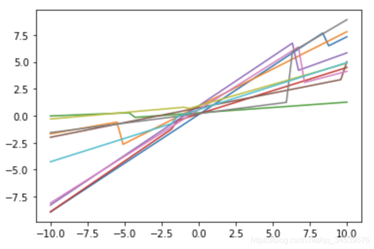
We can do it by simple 、 Basic modules , After repeated superposition , To implement more complex functions .
For more and more complex functions ? How do computers find derivatives ?
- What is machine learning ?
- KNN The disadvantages of this method , What is the background of linear fitting
- How to supervise , To get faster function weight updates
- The combination of nonlinear function and linear function , It can fit very complex functions
- We can learn deeply through basic function modules , To fit more complex functions
边栏推荐
猜你喜欢

220617,数据仓库dwd,

Towards Open World Object Detection

数据仓库dwb层,220620,hm,
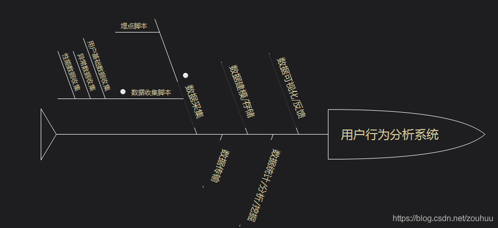
Building user behavior analysis system (I) -- Overview
review第1遍,220617,数据仓库DWD层,dwb层,视频,

XML file fuzzy query writing method SQL function find_ in_ set

大华海康摄像头视频拉流

OpenGAN: Open-Set Recognition via Open Data Generation

Renderdoc frame debugger

D2-多层神经网络的原理/神经网络自动求导的原理
随机推荐
[freeswitch development practice] over session limit 1000/locked, waiting on external entities
tensorRT
Review the first time, 220619, data warehouse DWB layer dimensionality reduction, video,
Multithreading - thread pool usage
Several commonly used databases of miRNA
Renderdoc frame debugger
Shadow Detection
DevOps失败了!
A Comparative Analysis of Deep Learning Approaches for Network Intrusion Detection Systems (N-IDSs)
Google Chrome cannot be installed successfully after uninstallation
论文阅读-Temporal Fusion Transformers for Interpretable Multi-horizon Time Series Forecasting
Join hands with Ziguang zhanrui to enter the Internet of things chip market with German communication through Hezhan microelectronics
Enumeration creation
根据url下载图片保存到本地 有问题请留言
三星S10系列配置售价曝光:5G版本定价或超万元!
Chinese garbled code problem of URL transmission in get request - collection "suggestions collection"
lc marathon 7.19
Leetcode thought notes for questions
Learning Placeholders for Open-Set Recognition
miRNA几大常用的数据库