Category loss

Cross Entropy Loss

Cross entropy loss can be divided into two categories loss and multi category loss

Two categories of losses

For dichotomies （ namely 0-1 classification ）, That is, it belongs to the third party 1 The probability of a class is p, Belong to the first 0 The probability of a class is 1−p. Then the binary cross entropy loss can be expressed as ：

After the unified format is ：

It can be understood as ： When the actual category is 1 when , We want the forecast to be category 1 The probability is higher , here $log(p)$ The greater the value of , The smaller the loss ; conversely , We want the forecast to be category 0 The probability is higher , here $log(1-p)$ The greater the value of , The smaller the loss . in application , The category probability of two categories is usually sigmoid Function maps the result to （0,1） Between .

Multi class loss

among ,$Y_i$ It's a one-hot vector , And defined as follows ：

$p_{ij}$ It means the first one i Three samples belong to the category j Probability . In practical application, we usually use SoftMax Function to get the probability that the sample belongs to each category .

derivative one-hot The establishment of vectors

• nothing num_classes

  import torch
  from torch.nn import functional as F
  
  x = torch.tensor([1, 1, 1, 3, 3, 4, 8, 5])
   
  y1 = F.one_hot(x) #  There is only one parameter tensor x
  print(f'x = ',x)  
  print(f'x_shape = ',x.shape) 
  print(f'y1 = ',y1)  
  print(f'y1_shape = ',y1.shape)
  

  Output ：

  x = tensor([1, 1, 1, 3, 3, 4, 8, 5])
  x_shape = torch.Size([8])
  y = tensor([[0, 1, 0, 0, 0, 0, 0, 0, 0],
          [0, 1, 0, 0, 0, 0, 0, 0, 0],
          [0, 1, 0, 0, 0, 0, 0, 0, 0],
          [0, 0, 0, 1, 0, 0, 0, 0, 0],
          [0, 0, 0, 1, 0, 0, 0, 0, 0],
          [0, 0, 0, 0, 1, 0, 0, 0, 0],
          [0, 0, 0, 0, 0, 0, 0, 0, 1],
          [0, 0, 0, 0, 0, 1, 0, 0, 0]])
  y_shape = torch.Size([8, 9])
  

• Yes num_classes

  y2 = F.one_hot(x, num_classes = 10)  #  here num_classes Set to 10, among  10 > max{x}
  print(f'x = ',x)  #  Output  x
  print(f'x_shape = ',x.shape)  #  see  x  The shape of the 
  print(f'y2 = ',y2)  #  Output  y
  print(f'y2_shape = ',y2.shape)
  

  result ：

  x =  tensor([1, 1, 1, 3, 3, 4, 8, 5])
  x_shape =  torch.Size([8])
  y2 =  tensor([[0, 1, 0, 0, 0, 0, 0, 0, 0, 0],
          [0, 1, 0, 0, 0, 0, 0, 0, 0, 0],
          [0, 1, 0, 0, 0, 0, 0, 0, 0, 0],
          [0, 0, 0, 1, 0, 0, 0, 0, 0, 0],
          [0, 0, 0, 1, 0, 0, 0, 0, 0, 0],
          [0, 0, 0, 0, 1, 0, 0, 0, 0, 0],
          [0, 0, 0, 0, 0, 0, 0, 0, 1, 0],
          [0, 0, 0, 0, 0, 1, 0, 0, 0, 0]])
  y2_shape =  torch.Size([8, 10])
  

difference ： No category specified , As given x Maximum +1 As the number of categories , Otherwise, press the specified num_classes draw one-hot vector

Focal Loss

The word is put forward in RetinaNet In the article , The purpose is to Pay more attention to those samples that are difficult to classify in training , It suppresses the leading role of those easy to classify negative samples . Address of thesis

Focal Loss It is an improvement of the typical cross information entropy loss function , For a dichotomous problem , The cross information entropy loss function is defined as follows ：（ It just said ）

In order to unify the loss function expression of positive and negative samples , First, make the following definition ：（ To put it bluntly $p_t$ Is the probability of the sample ）

$p_t$ Formally, it represents the confidence of the correct category predicted to correspond . In this way, the entropy loss of two classification cross information can be rewritten as follows ：

$\alpha$ Balance positive and negative samples

In order to balance the losses of most classes and a few classes , A conventional idea is to multiply the loss term by an equilibrium coefficient α∈(0,1), When the category is positive , take ${\alpha }_t=\alpha$, When the category is negative , take ${\alpha }_t=1-\alpha$, The cross information entropy loss with equilibrium coefficient obtained in this way is defined as follows ：

such , Select according to the number of positive and negative samples in the training samples $\alpha$ Value , We can balance the positive and negative samples . However , This does not differentiate between simple and difficult samples , In target detection , Balance most classes （ background ） And minority classes （ Prospects with goals ）, Also balance simple samples and difficult samples , The problem often encountered in the training process is that a large number of simple background samples occupy the main part of the loss function . therefore , It is also necessary to further improve the above cross information entropy loss with balance coefficient . So there was Focal Loss, It is defined as follows ：

$(1-p_t{)}^{\gamma }$ Balance difficult and easy samples

Compared with the above, the balance coefficient is added ${\alpha }_t$ Compared with the loss function ,Focal Loss There are two differences ：

• Fixed equilibrium coefficient ${\alpha }_t$ Replaced by a variable balance coefficient $(1-p_t)$
• There is another regulator $\gamma$, And $\gamma \ge 0$

analysis ：

• For samples with accurate classification （ That is to say Easy to separate samples , Positive sample $p$ Tend to be 1, Negative sample $p$ Tend to be 0）,$p_t$ Close to the 1,$1-p_t$ Close to the 0, It shows that the contribution to the loss is small , That is, it reduces the loss proportion of easily distinguishable samples , This is contrary to the original definition of cross entropy loss function ;
• For samples with inaccurate classification （ That is to say Hard sample , Positive sample $p$ Tend to be 0, Negative sample $p$ Tend to be 1）,$p_t$ Close to the 0,$1-p_t$ Close to the 1, It won't be right loss Too much impact , This is the same as the original definition of cross entropy loss function ;
• In the course of contacts , In a disguised way, the weight of samples with inaccurate classification in the loss function is improved （ Reduce classification accuracy , Although the inaccurate classification does not affect , In fact, it has been improved relatively ）
• $p_t$ It also reflects the difficulty of classification , $p_t$ The bigger it is , It shows that the higher the confidence of classification , It means that the easier the sample is to be divided ; $p_t$ The smaller it is , The lower the confidence of classification , It means that the more difficult it is to distinguish the samples . therefore focal loss amount to The weight of hard to distinguish samples in the loss function is added , Make the loss function tend to hard to divide samples , It helps to improve the accuracy of difficult samples .
• $\gamma$ be equal to 0 When , Just like the normal cross entropy loss function ,$\gamma$ The smaller it is , The more important the loss of hard to distinguish samples , The less important the easy sample is . The differences are given below $\gamma$ Of Focal Loss The loss function curve ：
  

$\alpha +\gamma$ combination

Obviously, both positive and negative samples are balanced , And balance the difficult and easy samples

Position loss

Location loss has L1 Loss,L2 Loss,Smooth L1 Loss（ Explain the multi-level target detection architecture in detail Cascade RCNN）,IoU Loss,GIOU Loss,DIoU Loss,CIoU Loss（ Detailed explanation IoU、GIoU、DIoU、CIoU、EIoU and DIoU-NMS）, These loss functions I mentioned in previous articles , Click to arrive at , I'll simply give the formula here .

L1 Loss

L2 Loss

Smooth L1 Loss

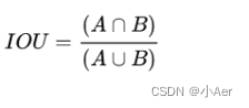
IoU Loss

GIOU Loss

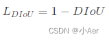
DIoU Loss

CIoU Loss

Inference

[0] https://blog.csdn.net/sinat_34474705/article/details/105141134
[1] https://zhuanlan.zhihu.com/p/266023273
[2] Hard samples and positive and negative samples
[3] https://blog.csdn.net/BIgHAo1/article/details/121783011